Aim of the Study

This study aims to understand the thermal influence of an urban forest tree canopy using the LES model PALM. The study analyses different spatial densities of tree spacing to assess which density brings most daytime/ nighttime cooling/ heating due to the shading of the tree canopy and the evapotranspiration effect. 

PALM-4U Simulation Domain

COSMO Data Acquisition

The COSMO D2 analysis data that was use to produce the dynamic_driver data for PALM was obtained via the online Pamore API service.

"-flow" data request:

The command: pamore -d 2018080600 -de 2018081100 -model cd2_ana -lt ass -suffix "-flow"




Retrieved the following data:

QNV-request oflxd21.8cc8427d6b8026c1a7dc59f0a595bff0003 ended successfully

command: pamore -d 2018080600 -de 2018081100 -model cd2_ana -lt ass -suffix "-flow"

location of the data - host:            download.dwd.de
                       directory:       pub/Pamore/oflxd21.8cc8427d6b8026c1a7dc59f0a595bff0003
                       available until: 17.10.2023

                       link:            https://download.dwd.de/pub/Pamore/oflxd21.8cc8427d6b8026c1a7dc59f0a595bff0003

ACCOUNTING of QNV-DATABASE-REQUEST
----------------------------------
req-ID                                      user           sended              execute       realtime dbreq  gribs    MByte pamore-command
------------------------------------------- -------- ------------------- ------------------- -------- ----- ------ -------- --------------
oflxd21.8cc8427d6b8026c1a7dc59f0a595bff0003 xxxxxxxx 09.10.2023 16:43:09 12.10.2023 03:25:12      169   121  92969    79153 '-d 2018080600 -de 2018081100 -model cd2_ana -lt ass -suffix "-flow"'

  

"-soiltype" Data Request

The command: pamore -d 2018080600 -hstop 0 -ee SOILTYP -model cd2 -lt ass -suffix "-soiltype"

Retrieved the following data:

QNV-request oflxd21.76cd14673b8dcbb1fdf43903aa38345e000 ended successfully

command: pamore -d 2018080600 -hstop 0 -ee SOILTYP -model cd2 -lt ass -suffix "-soiltype"

location of the data - host:            download.dwd.de
                       directory:       pub/Pamore/oflxd21.76cd14673b8dcbb1fdf43903aa38345e000
                       available until: 16.10.2023

                       link:            https://download.dwd.de/pub/Pamore/oflxd21.76cd14673b8dcbb1fdf43903aa38345e000

ACCOUNTING of QNV-DATABASE-REQUEST
----------------------------------
req-ID                                      user           sended              execute       realtime dbreq  gribs    MByte pamore-command
------------------------------------------- -------- ------------------- ------------------- -------- ----- ------ -------- --------------
oflxd21.76cd14673b8dcbb1fdf43903aa38345e000 xxxxxxxx 09.10.2023 16:12:17 11.10.2023 02:29:32        2     1      1        0 '-d 2018080600 -hstop 0 -ee SOILTYP -model cd2 -lt ass -suffix "-soiltype"'

"-hhl" Data Request

The command: pamore -d 2018080600 -hstop 0 -ee SOILTYP -model cd2 -lt ass -suffix "-soiltype"

Retrieved the following data:

QNV-request oflxd21.46795a029091707a73ac2458292f83e9002 ended successfully
command: pamore -d 2018080600 -ee HHL -model cd2 -lt ass -suffix "-hhl"

location of the data - host:            download.dwd.de
                       directory:       pub/Pamore/oflxd21.46795a029091707a73ac2458292f83e9002
                       available until: 14.10.2023

                       link:            https://download.dwd.de/pub/Pamore/oflxd21.46795a029091707a73ac2458292f83e9002

ACCOUNTING of QNV-DATABASE-REQUEST
----------------------------------
req-ID                                      user           sended              execute       realtime dbreq  gribs    MByte pamore-command
------------------------------------------- -------- ------------------- ------------------- -------- ----- ------ -------- --------------
oflxd21.46795a029091707a73ac2458292f83e9002 xxxxxxxx 06.10.2023 14:06:32 09.10.2023 09:16:42        3     2    132      138 '-d 2018080600 -ee HHL -model cd2 -lt ass -suffix "-hhl"'

INIFOR Data Processing

The data was then processed using the INIFOR pre-processor native to PALM

The following command produced the thf_base_2018080700_dynamic file:

inifor --path /mnt/d/phd/thf/data/cd2_ana/download/nc/flow --date 2018080700 --init-mode profile --soil-init-mode volume -s /mnt/d/phd/thf/data/cd2_ana/download/nc/flow/soil.nc -t /home/joshuabl/palm/current_version/JOBS/thf_base/INPUT/thf_base_static -n /home/joshuabl/palm/current_version/JOBS/thf_base/inifor/namelist -o /home/joshuabl/palm/current_version/JOBS/thf_base/INPUT/thf_forest_5m_dynamic.nc --soil-prefix laf_ --input-prefix laf_

Generate the Validation Plot

Below shows a comparison of air temperature values for the PALM baseline simulation, DWD weather data, and PALM dynamic_driver (COSMO D2 analysis) Here is the file the reproduce the plot below: thf_forest_dwd_validation.ipynb 

COSMO Data Download:

Domain Size

Number of grid cells=nx, ny, nz
Grid cell size=dx, dy, dz

Parent domain:

Parent Domain

Child Domain (N02)

Weather Station vs PALM Simulation 

Air temperature validation of DWD weather station data:

station_id	dataset	parameter	date	value	quality	from_date	to_date	height	latitude	longitude	name	state
00433	temperature_air	temperature_air_mean_200	2018-08-07 00:00:00+00:00	293.55	3.0	1951-01-01 00:00:00+00:00	2024-01-31 00:00:00+00:00	48.0	52.4676	13.402	Berlin-Tempelhof	Berlin

 

Validation Plot

The following figure shows air temperature (degrees celsius) over two duranial cycles from the date 2018-08-07 00:00:00+00:00 to 2018-08-09 00:00:00+00:00. Here is a link to the Python code to reproduce the plot: thf_forest_dwd_validation.ipynb. The PALM NetCDF file used in the validation plot can be downloaded here: thf_base_2018080700_av_3d_merged.nc

Spatial Details of the horizontal slice

latitude = 52.4676
longitude = 13.402

Discussion 

As you can see there is an acceptable fit between the Tempelhofer Feld weather station and the PALM baseline simulation. Note that the DWD weather (orange line)  contains one extra timestep at the start of the time series 2018-08-07 00:00:00+00:00 compared with the PALM baseline simulation (blue line). This is due to the fact that PALM was set to output data after the first time step, in this case 2018-08-07 01:00:00+00:00 (1am). 

The PALM simulation displays some latency behind the DWD weather data. This could be due to an a spatial temporal difference as the PALM domain contains a 10m terrain step near the site of the weather station. However, the sensor is upwind from the terrain step in the simulation domain and should not have any significant influence on the results. Another explanation could be due to insufficient surface spinup time (48hrs) of the PALM model surfaces. Therefore introducing some latency to reach real world temperatures. 

OUTPUT Files:

Comparison Plot

Please be aware that only case "thf_base_2018080700" contains the OUTPUT data directory. This is due to the size of each case (64G) and data storage constraints. However validation analysis can be undertaken using the "thf_base_2018080700" case.

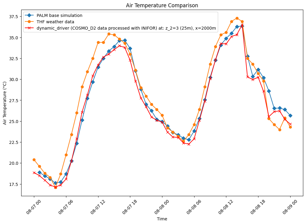
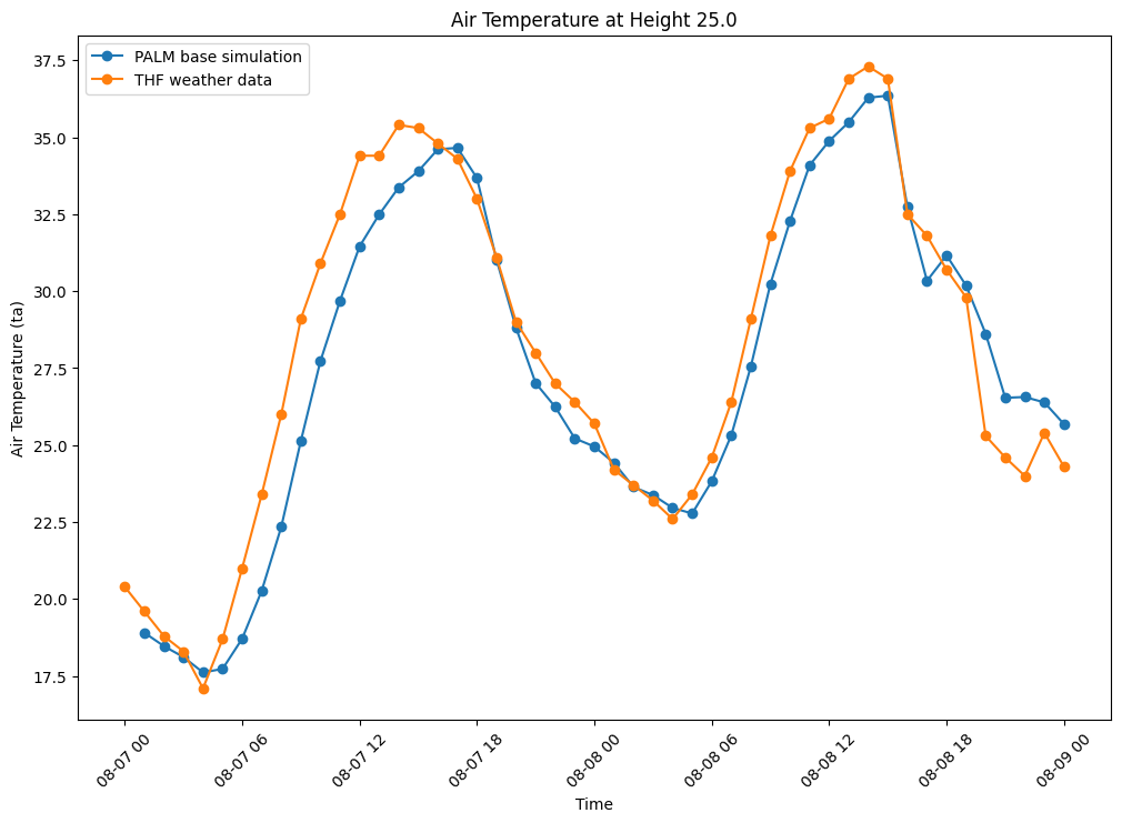
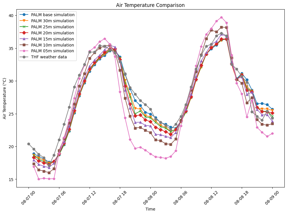
The following figure shows air temperature (degrees celsius) over two duranial cycles from the date 2018-08-07 00:00:00+00:00 to 2018-08-09 00:00:00+00:00. This time all tree spacing cases have been included in the plot to cross compare the results. 

Here is a link to the Python code to reproduce the plot: thf_forest_ta_case_comparison.ipynb

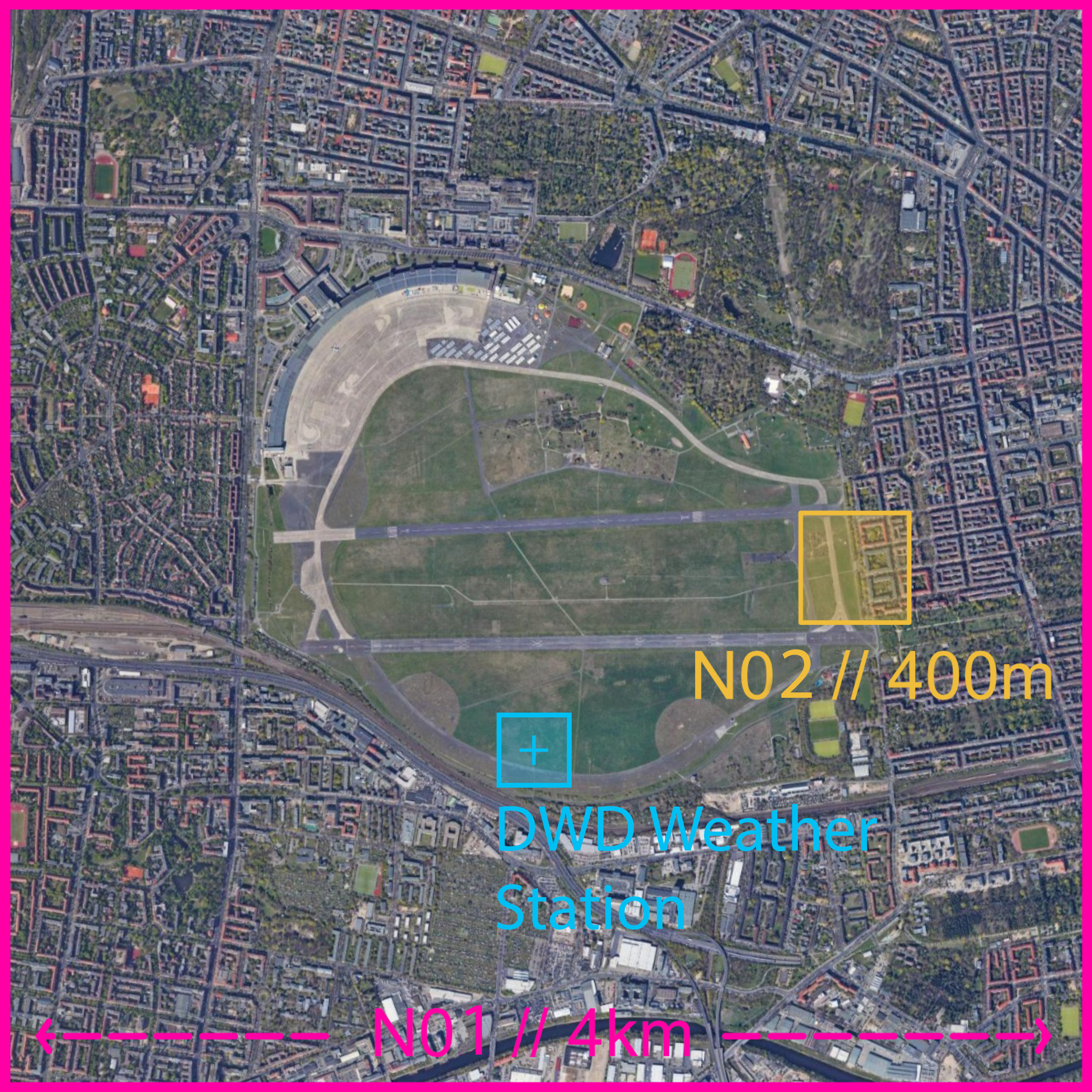
The location of the validation point was set to (DWD weather station):

Discussion

These results must be taken with much caution as full validation of the PALM Plant Canopy Model (PCM) (specifically 3D single trees) has not yet been validated. However the validation of a 2D forest patch with the PALM PCM has been undertaken - for example Paleri et al. (2023). The following discussion is just speculation based on preliminary results. I encourage the PALM developers involved in the PCM to engage in this discussion to help validate the result. 

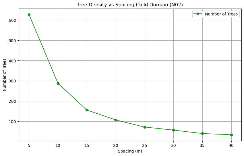
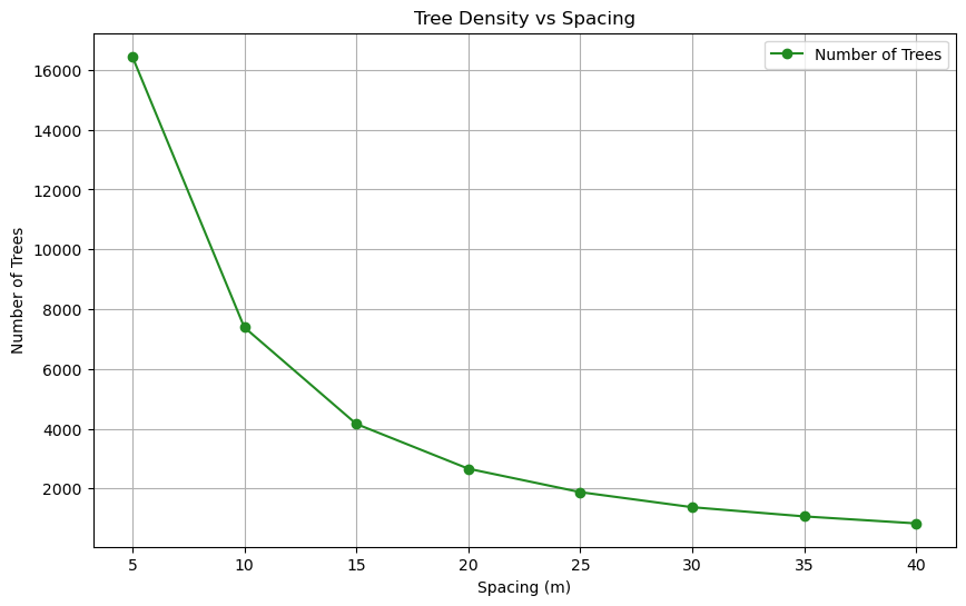
The results show that increasing tree density lowers nighttime temperature and increases daytime temperatures, compared with the baseline (blue line) and weather station data (grey line). Some explanation for the exponential nighttime cooling effect, for example the low temperatures at 08-08-00, case 05m (10m tree spacing trunk to trunk - pink line), in comparison to the other cases might be due to the exponential increase in trees, thus more shading and evapotranspiration effect as can be seen by the exponential curve of trees added at each density in following figure:

Potential Sources of Error

One potential issue that might cause hightended cooling of nighttime air temperature in the tree canopy is the following setting in the p3d file: 

 
Another case without the cloud model is needed to be run in order to rule out this possible cause of unrealistically low air temperatures.

Another source of error could be due to using the single trees in a domain with large grid spacing (10m in this case). It is recommended in the PALM documentation to only use single tree with LAD and BAD profiles when the level of detail (LOD1) is less than a 1m grid resolution. Although, the same air temperatures can be found in the child domain (N02). Suggesting that grid sensitivity to the single trees in PALM is not the main cause of error. This cannot be proven until another case is run with a 1m grid resolution in the child domain.

Specifying the full range of tree options via the palm_csd Python script is needed to make sure the trees in the study are specified correctly. Below is a list of possible single tree options available:

Index	|=Species	Shape	Crown height/width ratio(*)	Crown diameter (m)	Height (m)	LAI summer(*)	LAI winter(*)	Height of maximum LAD (m)(*)	LAD/BAD ratio(*)	DBH (m)
0	Default	1.0	1.0	4.0	12.0	3.0	0.8	0.6	0.025	0.35
1	Abies	3.0	1.0	4.0	12.0	3.0	0.8	0.6	0.025	0.80
2	Acer	1.0	1.0	7.0	12.0	3.0	0.8	0.6	0.025	0.80

Currently only the following tree options have been switched on as you can see in this example CSV array:


Crown height/width ratio(*), DBH, Height of maximum LAD (m)(*), LAD/BAD ratio(*) and DBH (m) are still yet to be utilised!

Feedback from the PALM developers and personnel responsible for maintaining the PALM Plant Canopy Model and palm_csd Python Processor would be most welcome. I believe that a thorough investigation and validation of the PMC would also be beneficial to the PALM community and scientific users.

Download Files

All the data for this study is openly available via the following links for reproducibility:

Please be aware that only case "thf_base_2018080700" contains the OUTPUT data directory. This is due to the size of each case (64G) and data storage constraints. However validation analysis can be undertaken using the "thf_base_2018080700" case.

Leaf Area (LA), Leaf Area Index (LAI), Leaf Area Density (LAD), and Basal Area Density (BAD) are all metrics used in forestry and environmental science to quantify vegetation structure and canopy characteristics. Here’s how they differ and how they’re typically measured and calculated:

Leaf Area (LA):

• Description: The total leaf surface area of a plant or group of plants.
• Measurement: Direct measurement involves collecting and scanning leaves to determine their area with specialized software. Indirect methods include using leaf mass and specific leaf area (SLA, the area per unit mass).
• Equation: ( LA = \sum (\text{Individual Leaf Areas}) )
• Python Representation: python leaf_areas = [5.0, 3.5, 4.2] # Example areas in square meters total_leaf_area = sum(leaf_areas)

Leaf Area Index (LAI):

• Description: The area of leaves per unit ground surface area. It’s dimensionless and provides a measure of canopy coverage.
• Measurement: Can be measured using indirect methods like hemispherical photography, ceptometers, and LAI meters, which calculate LAI from light transmission through the canopy.
• Equation: ( LAI = \frac{\text{Total Leaf Area}}{\text{Ground Area}} )
• Python Representation: python ground_area = 100 # Example ground area in square meters lai = total_leaf_area / ground_area

Leaf Area Density (LAD):

• Description: The leaf area per unit volume of space. It’s used to describe the vertical distribution of leaves within a canopy.
• Measurement: Often derived from LAI and canopy height using models, or measured directly using LIDAR or destructive sampling where leaves are collected at different canopy heights.
• Equation: $$ LAD(z) = \frac{\text{dLA}}{\text{dV}} $$ where ( \text{dLA} ) is the differential leaf area in a small volume ( \text{dV} ) at height ( z ).
• Python Representation: python def calculate_lad(la, canopy_volume): return la / canopy_volume

Basal Area Density (BAD):

• Description: The cross-sectional area of the tree trunk(s) per unit ground area, often at breast height (1.3 m). It’s an indicator of forest stand density.
• Measurement: Measured using a diameter tape or calipers at breast height and then calculating the area. For whole stands, a relascope or angle gauge is used to sample basal area per unit area.
• Equation: ( BAD = \frac{\pi \times (\text{DBH}/2)^2}{\text{Ground Area}} ) where DBH is Diameter at Breast Height.
• Python Representation: python def calculate_bad(dbh, ground_area): radius = dbh / 2 return np.pi * (radius**2) / ground_area

In terms of data collection methods: - Direct Measurements: Physically measuring the leaves, branches, and trunks using tapes, calipers, etc. - Indirect Measurements: Using optical instruments or remote sensing technologies that infer the metrics from light transmission, reflection, or absorption.

When represented in Python, these metrics can be calculated using functions that take the necessary parameters (like leaf areas, tree DBH, canopy volume, etc.) and perform the corresponding arithmetic operations, as shown in the pseudo-code examples above. For actual data analysis, you’d need arrays or datasets containing these parameters, often collected in the field or derived from remote sensing imagery.

$$\textrm

{Workaround to have inline math:} \alpha \times \Pi} \over {\gamma \textrm

{however, I wish to have better solution} $$